I live in Italy, and more precisely in Milan, a city known for fashion and design events. During a lunch break I was visiting the Pinacoteca di Brera, a 200 centuries old museum. This museum is full of incredible paintings from the Renaissance period. During my visit I was particularly impressed from one of them: “La Vergine con il Bambino, angeli e Santi”, by Piero della Francesca.

If you see this painting you will find a profound of colours with a great equilibrium between different hues, the hardy usage of complementary colours and the ability expressed in the “chiaroscuro” technique. While I was looking at the painting I started, wondering how we moved from this wisdom to the ugly charts you can easily find within today’s corporate reports ( find a great sample on the WTF visualization website) This is where Paletter comes from: bring the Renaissance wisdom and beauty within the plots we produce every day.
Introducing paletter
PaletteR is a lean R package which lets you draw from any custom image an optimized palette of colours. The package extracts a custom number of representative colours from the image. Let’s try to apply it on the “Vergine con il Bambino, angeli e Santi” before looking into its functional specification.
Installing paletter
Since paletteR is available only trough Github we have to install it using devtools:
library(devtools)
install_github("andreacirilloac/paletter")
Creating a palette from your image
to draw our palette we now need to:
_image_path_
_number_of_colours_
_type_of_variable_
Here it is the code (you can donwload the picture from wikicommons visiting https://it.wikipedia.org/wiki/File:Piero_della_Francesca_046.jpg):
create_palette(image_path = "~/Desktop/410px-Piero_della_Francesca_046.jpg",
               number_of_colors =20,
               type_of_variable = “categorical")
and here it is the output:
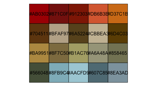
As you see the palette drawn contains all the most representative colours, like the red of the carpets or the wonderful blue of San Giovanni Battista on the left of the painting.
Functional specification
The main idea behind paletteR code is quite simple:
kmeans
Let ’see how all this works in brief.
Reading a picture into the RGB colourspace
This first step involves transforming the image into an abstract object on which we can apply statistical learning. To do so we read the image file and convert it into a three multidimensional matrix. Within the matrix to each image pixel three numbers are associated:
All those three attributes range from 0 to 255, as requested by the rules of the RGB colourspace ( find out more on the related RGB colourspace page on wikipedia) . To perform this transformation we use the readJPEG() function from Jpeg package:
painting <- readJPEG(image_path)
this will generate an array having for each point within the image both the cartesian coordinates and the R, G and B values of the related colours. We now apply some statistical learning on the array, to select most representative colours and create an optimized palette.
Processing the RGB image trough kmeans
This processing step was actually the first developed of the package and I already described it in a previous post. Within tht post I devoted the right time to expose some theoretical reference to the kmeans algo and it application to images. Please refere to the How to build a color palette from any image with R and k-means algo post to get a proper explanation of this. You can also read more about this algo and its inner rationales within R for data mining a data mining chrime book. What we need to repeat here is that by applying the kmeans algo on the array we get a list of RGB colours, selected as the most representative of the ones available within the image. I clearly remember my feeling when the first palette came out of kmeans: it was thrilling, but the results were undeemebly poors. I came out for instance with this:
What was wrong with the palette employed? We can pick at least three answers:
- there are too bright colours
- there are too dark colours
- there are too similar colours
To summarise: my package was stupid, it was unable to reasonate about relationship among colours avaiable. To solve this problem I moved to the hsv colour space which is the perfect environment were to perform such kind of analyses. the HSV colourspace expresses every colour in terms of:
- Hue, which properly expresses the colour, and gets a value from 0 to 360
- Saturation, which expresses the quantity of colour (think about a pigment diluted with water to get it). This takes a value from 0 to 100%
- Brightness or Value, which express the quantity of grey or white included within the colour. This also takes a value from 0 to 100%
The way HSV system describes colours makes it easy to sort colours, moving from 0 to 360, and check for too bright or too dark colours, analysing distributions of saturation and brightness. You can get more on this on the really detailed Wikipedia page of HSV
Moving to the hsv colours space
To convert our RGB object into the HSV space we just need to apply rgb2hsv() to the values of R, G and B.
Removing outliers
What would you do next? After moving within the HSV realm we can now draw meaningful representations of our colour data. What paletteR does as a first step is to produce descriptive statistics for values of Saturation and Value. First of all we calculate quartiles of all of those values:
brightness_stats <- boxplot.stats(sorted_raw_palette$v)
saturation_stats <- boxplot.stats(sorted_raw_palette$s)
Once being done with that we remove the lowest and highest of both. This lets us fix the first two problems observed in the first palette: too bright and too dark colours. What about the third problem?
Optimising palette
To get this solved we have to reasonate about the visual distance of colours. Look for instance at those colours? ! You would definitely say the first and the second are more distant from each other than the second and the third. You would definitely be right, but how to make our PaletteR as cleaver as you? This is simply done within the HSV space leveraging the Hue attribute. As we have seen HSV hues are placed along a circle in a visually reasonable way. This means that a hue of 40 (which is some kind of orange) is way more distant from a hue of 100 (green) than a hue of 90 is ( another green). Knowing this we just have to select from the first set of colours coming from kmeans a second subset of colours selected as the most distant. This will let us avoid employing colours appearing too similar. How to do this? The current version of paletteR does it:
- generating a random sample of possible alternative palettes
- measuring the median distance among hues within the palette
- selecting the palette showing the greatest distance
And here it is below the result for our dear Renaissance painting:
Isn’t that better than the previous one?
How to apply paletteR in ggplot2
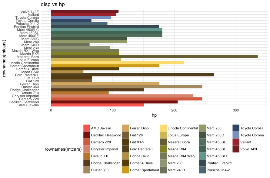
Applying the obtained palette in ggplot is actually easy. The object you obtain from the _create_palette_ function is a vector of hex codes (another way of codify colours, more on the Wikipedia page). You therefore have to pass it to your ggplot plot employing scale_color_manual().A small side note: be sure to select a number of colours equal to the number of variables to plot. Let’s apply our palette by Raffaello with an hyphotetical plot:
colours_vector <- create_palette(image_path = image_path,
number_of_colors =32,
type_of_variable = “categorical")
ggplot(data = mtcars, aes(x = rownames(mtcars),y = hp,color = rownames(mtcars),
                          fill = rownames(mtcars))) +
  geom_bar(stat = 'identity') +
  scale_color_manual(values = colours_vector) +
  scale_fill_manual(values=colours_vector)+
  theme_minimal() +
  guides(size = FALSE) +
  theme(legend.position = "bottom") +
  labs(title = "disp vs hp")+
  coord_flip()
Which will produce:
Join us
paletter is quite a young package, nevertheless it already catched some interest (I was also invited to give a speach about it, you can watch it online.
Also the well known dataviz expert Alberto Cairo pointed it out as an useful tool:
Ohhh, an R library that detects colors in pictures. I can see this being useful for many projects https://t.co/m2TPshm5e0 #dataviz #infographics #ddj pic.twitter.com/yL5DbwygFc
— Alberto Cairo (@albertocairo) May 8, 2018
This is because of:
- its simple and rather powerful application of statistical learning to the color space
- the flexible code
- the high number of possible use cases
Since it is a young package there is still some work to do on it. I can see at least the following areas where further improvements could be introduced:
Would you like to give an help on this? Welcome on board! You can find the full code on Github and every contributions is welcome.